
During our previous lesson, we discovered that when you first gaze upon the night sky, you’ll notice that stars come in various colors. However, it’s not just the color and temperature of stars that can differ. Scientific observations have revealed that many stars exist as pairs or are part of intricate systems. In this current lesson, we will delve into the realm of double stars. We will explore the different types of double stars and examine the laws that govern the movements of stars in binary systems. Additionally, we will discover how to accurately determine the masses of stars.
Currently, it is not possible to watch or distribute the instructional video to students
In order to have access to this and other video lessons included in the package, you will have to add it to your individual account.
Obtain extraordinary functionalities


Outline for the Lesson “Determining the Mass of Stars: Binary Stars”
In the previous lesson, we discovered the vast diversity of stars. When first exploring the night sky, one cannot help but notice the varying colors of the stars. This distinction becomes even more apparent when examining their spectra. By analyzing the types of spectral lines and their intensity, we can classify stars based on their temperature, ranging from class O to class M, which reflects a decrease in atmospheric temperature.
However, stars can be differentiated not only by their color and temperature. Observations have revealed that many stars exist in pairs or as part of complex systems. In fact, approximately half of all stars in our Galaxy are part of double systems.
Binary stars are pairs of stars that are in close proximity to each other.
Among the stars that appear adjacent to each other in the night sky, there are two types of doubles: optical doubles and physical doubles. Optical doubles are stars that appear to be next to each other when projected onto the celestial sphere, but they may actually be located far apart from each other in reality.
On the other hand, physical double stars are indeed located near each other in space. They are not only bound together by the force of gravity, but they also orbit around a common center of mass.
The concept of double stars was first proposed by the English scientist and clergyman John Michell in 1767. Observational evidence supporting this hypothesis was later published by William Herschel in 1802.
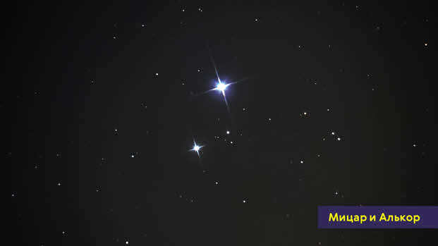
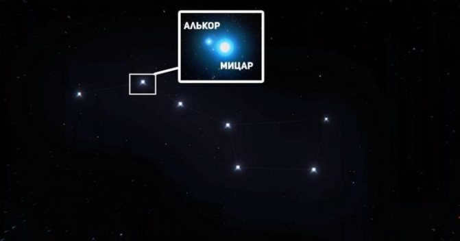
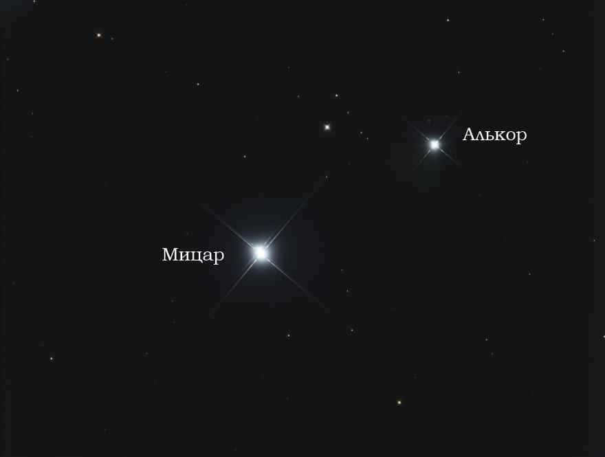
Mizar and Alcor, located in the handle of the Big Dipper, have been recognized as the earliest known star pair dating back to ancient times. These stars serve as a prime example of an optical double star, with Alcor positioned approximately 12 arc minutes apart from Mizar.
However, when observing Mizar through a telescope, one can easily discern its dual nature, as it is composed of two closely located stars known as Mizar A and Mizar B. This particular stellar pair serves as an illustration of a physical binary star.
When the number of stars within a system, bound together by the force of gravity, surpasses two, they are referred to as multiples. These multiples can take the form of triple, quadruple, or even higher configurations. An example of a multiple star is the triple star α Centauri. Interestingly, one of its components, Proxima, holds the distinction of being the closest star to Earth, second only to our own Sun.
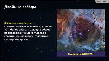
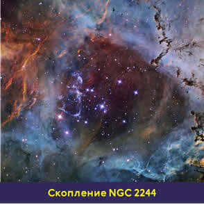
Multiple stars are defined as systems containing fewer than 10 components. If a system exceeds this limit, it is classified as a star cluster. A prime example of such a cluster is the Pleiades cluster, which can be observed with the naked eye in the night sky.
Physical binary stars, depending on the method of observation, are typically classified into various categories. Let us examine them in detail.
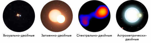
Stars that can be observed as visually double stars. are double stars where the individual components can be seen separately, either through a telescope or in photographs. The ability to observe a star as a visual double star depends on the resolving power of the telescope being used. As a result, all visually double stars that have been identified so far are located relatively close to the Sun and have extremely long orbital periods, lasting up to several thousand years. In fact, the orbits of these stars are similar in size to the orbits of the giant planets in our own solar system. Due to these factors, out of the over 110,000 visually double stars that have been discovered, less than a hundred have had their orbits accurately determined.
It has been discovered that the components of double systems exhibit a relative apparent motion that can be described as an ellipse and adheres to the law of areas. As a result, the orbits of stars in double systems follow Kepler’s laws and are governed by Newton’s law of universal gravitation.
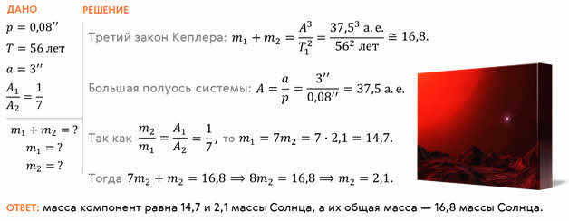
Consequently, by applying the third generalized law of Kepler to these systems at a known distance, we can determine their mass. This can be achieved by comparing the satellite motion of a star with the motion of the Earth around the Sun.
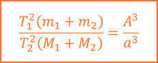
If we assume that the mass of the Sun is one unit and the major semi-major axis of the Earth’s orbit is one astronomical unit, and if we disregard the mass of the Earth in comparison to the mass of the Sun, we can calculate the total mass of the binary system in terms of solar masses using a certain ratio:
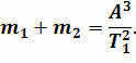
If we need to calculate the mass of each component in a pair of stars, we must examine the movement of each star and determine their distances from the shared center of mass:
Then, the ratio of the component masses in the star pair will be inversely proportional to the ratio of their orbit’s major semi-axes:
As an example, let’s find the total mass and stellar masses of a binary star with an annual parallax of 0.08”. Let’s assume that the orbital period of the components is 56 years and the major semi-axis of the apparent orbit is 3”. The distances of the star components from the center of mass are in a 1:7 ratio.
Observations of binary stars and the determination of their masses for various types have revealed the following:
– The masses of the stars range from 0.03 to 60 solar masses. The majority of stars fall within the mass range of 0.4 to 3 solar masses;
– There is a correlation between the masses of stars and their luminosities, allowing for the estimation of the masses of individual stars. For stars with masses ranging from 0.5 to 10 solar masses, their luminosity is proportional to the fourth power of their mass. For stars with masses exceeding 10 solar masses, the relationship is quadratic.
The second category of double systems is referred to as eclipsing-double or eclipsing-variable stars. These stars consist of closely orbiting pairs with a period ranging from several hours to several days. The size of their orbits is comparable to the size of the stars themselves, resulting in a very small angular distance between the stars. As a result, the individual components of the system cannot be observed separately.
However, the dual nature of the system can be inferred from the periodic fluctuations in its brightness. If the planes of the stars’ orbits are nearly aligned with the line of sight, eclipses can be observed as one component passes in front of or behind the other during their orbit.
The term used to describe the difference between the magnitudes at the smallest and largest points is known as amplitude. Additionally, the duration between two consecutive lowest points is referred to as the period of variability.
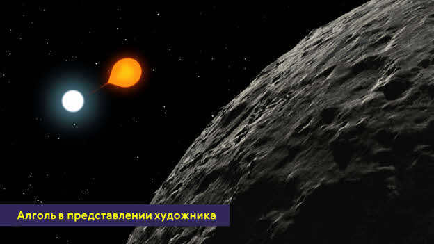
An iconic illustration of a variable star that undergoes eclipses is β Perseus (Algol). Algol experiences a period of eclipse lasting for 9.6 hours every 2.567 days.
There are currently around 4000 known eclipsing double stars.
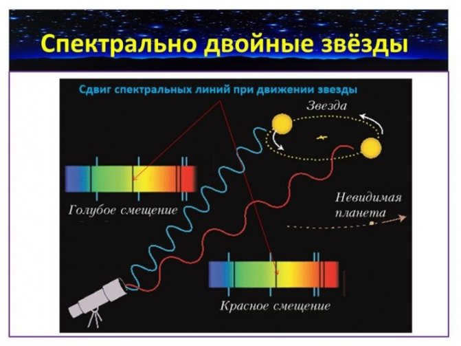
The next category is made up of spectrally double stars. These are stars that are determined to be double based solely on spectral observations.
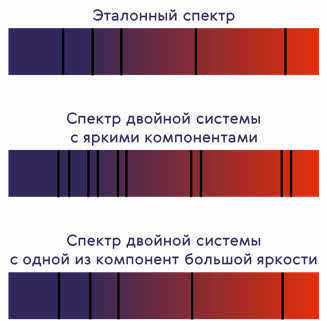
Let’s consider a scenario where we have two stars: one is a bright and massive star called A, and the other is a less bright but still massive star called B. Both stars orbit around a common center of mass, sometimes moving closer to the observer and other times moving farther away.
Because of the Doppler effect, when the stars are approaching the observer, the spectral lines will shift towards the violet region of the spectrum. Conversely, when the stars are moving away, the lines will shift towards the red region. The period of these shifts corresponds to the period of the stars’ rotation.
What is intriguing is that this technique led to the discovery of a satellite around the star 51 Pegasus in 1995. This satellite had a mass approximately equal to half the mass of Jupiter. This event marked the identification of the first exoplanet (which is the term used for planets outside our solar system).
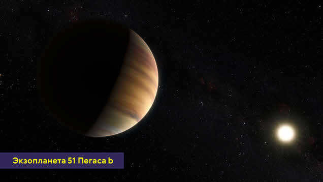
As of mid-October 2017, the spectral method has reliably confirmed the presence of 3,672 exoplanets in 2,752 planetary systems.
Furthermore, there is another category of double systems known as astrometrically double stars. These are binary star systems in which one star is either significantly smaller or has a lower luminosity.
The presence of a companion star in such a system can only be detected by observing the deviations of the brighter star from its straight path. These deviations have been found to be proportional to the mass of the companion.
Approximately 20 astrometrically double systems have been identified among stars that are in close proximity to the Sun.

I have created two videos discussing double and multiple stars. This is the second installment, which focuses on the various classes of stars that can form part of double and multiple systems, their interactions, and provides examples of different combinations, including the most rare and exotic ones. You can also check out the first part:
14.9K posts 45.3K followers
Community Guidelines
What guidelines can there be here, other than the guidelines set by the peekaboo itself 🙂
Wow, I just subscribed to your channel. I didn’t expect to see you here))))
Yeah, it’s fascinating. “She has a light bulb inside her.”
On August 18, 2023, at 00:01, Saturn will be visible in the constellation of Orion.
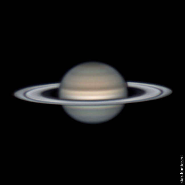
My gear:
-I used a Sky-Watcher Dob 14 (350/1600) Retractable SynScan GOTO telescope
-I also had a Lens Barlow NPZ PAG 3-5x
-To correct for atmospheric dispersion, I used a ZWO ADC (atmospheric dispersion corrector)
-I had a ZWO IR-cut light filter to enhance the quality of the images
-For capturing the astronomical images, I used a ZWO ASI 183MC camera.
Location: I was at the Caucasus Mountain Observatory, which is part of Moscow State University in the Karachay-Cherkess Republic.
Here is a snippet from the original video clip:

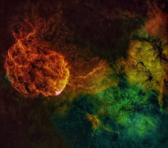
The Jellyfish Nebula captured using three narrowband filters
Various Perspectives of the Milky Way
Latest discovery: Comet C/2023 P1 (Nishimura)
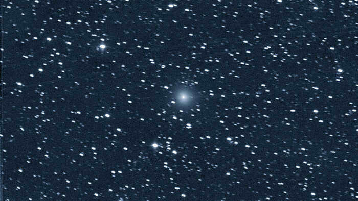
Comets are unexpected visitors. While the old ones, which we have known for a long time, can be disappointingly predictable (which is not surprising, as they have had time to deplete and melt during repeated approaches to the Sun), newly discovered comets are often dazzlingly bright and spectacular. However, this is not always the case.
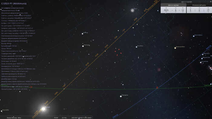
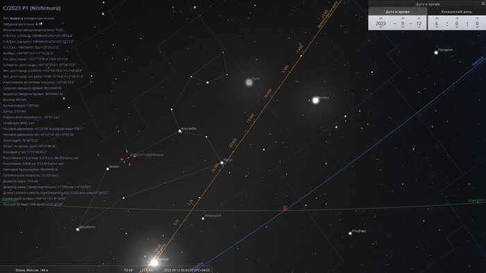
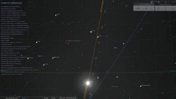
The location of comet C/2023 P1 in the constellation Gemini (when it was first observed) on the morning of August 12, 2023.
However, the brightness of the comet increased with each passing night. And now, just one week later, it has already achieved a magnitude of 10 stars. It is now visible through medium-power amateur telescopes. Although Nishimura’s comet is still best seen before dawn, the overall viewing conditions have improved slightly since its initial discovery.
What Comes After?
On September 18, 2023, the comet will reach perihelion (the point in its orbit closest to the Sun), coming within a distance of 33 million kilometers from its luminous surface. That’s roughly twice as close as Mercury. However, unlike Mercury, which is a solid rock, the comet is composed of ice, which will start to melt and vaporize well before reaching perihelion. This process is already underway, and astronomers have observed a small tail (measuring only 8-10 angular minutes in length) consisting of gases and dust emitted from the comet’s heated nucleus.
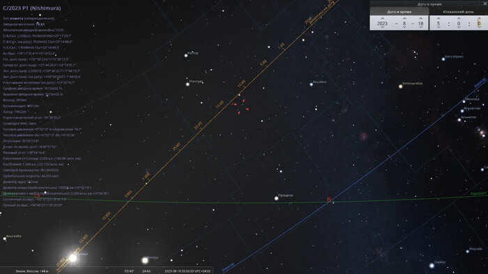
On the morning of August 18, 2023, the comet C/2023 P1 can be found in the Gemini constellation.
Currently, the comet is traversing the Earth’s orbit and is positioned on the opposite side of the Sun. As a result, the distance between the Earth and the comet is quite significant, measuring one and a half astronomical units. However, this situation is rapidly changing.
By the beginning of September, the comet will be only 1 astronomical unit away from Earth (and only ½ ae away from the Sun). Although the angle between the Sun and the comet will slightly decrease (from 35 to 30 degrees), this will be offset by the increasing difference in declination. In fact, the comet’s tail will be visible directly above the Sun, allowing for a clear view of it before sunrise.
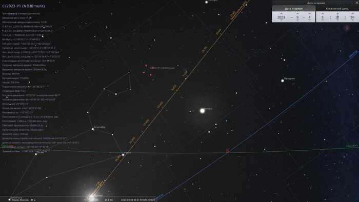
In the sky, on September 4, 2023, the comet C/2023 P1 will be positioned in the constellation of Cancer. It will be located near the border with the constellation of Leo, specifically near the asterism known as “Lion’s Head,” which serves as a great reference point. Additionally, the bright planet Venus will also be visible in the same constellation. This day, the comet will shine with a brightness of the 7th magnitude, making it an easily observable object when using binoculars.
By the morning of September 9, 2023, comet C/2023 P1 will be found just 1 degree west of the star Adhafera (Zeta Leo), with a brightness reaching the 6th magnitude. In regions with ideal conditions such as mountains, deserts, or steppes, the comet will even be visible to the naked eye.
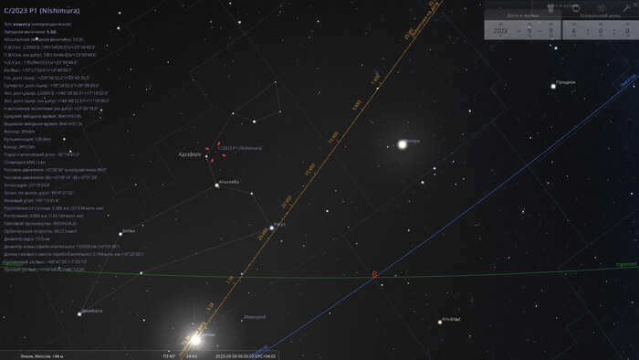
The comet C/2023 P1 will be located in the constellation Leo on the morning of September 9, 2023.
Unfortunately, the distance from the Sun will decrease to 22 degrees, but the comet will rise even higher above the ecliptic. Despite this small elongation, the comet will be visible for at least one and a half to two hours.
In the upcoming days, the brightness of the comet will continue to increase, but the distance from the Sun will decrease, making observation more challenging.
By the morning of September 12th, the comet’s brightness will reach a magnitude of 5 stars, and its elongation will decrease to 17 degrees. Meanwhile, the comet will still be positioned above the Sun, providing an opportunity to spot it in the early morning light near the star Zosma (Delta Leo).
The location of comet C/2023 P1 in the Leo constellation on the morning of September 12, 2023
During the morning of September 15, the comet will come close to the 2nd magnitude star, Denebola (Beta Leo). At the same time, the comet itself will be just slightly dimmer, with a stellar magnitude of around 3rd. However, it will be challenging to observe both celestial objects against the relatively bright dawn sky.
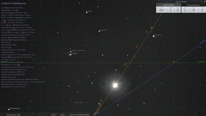

On September 15, 2023, in the morning, comet C/2023 P1 will be located in the Leo constellation
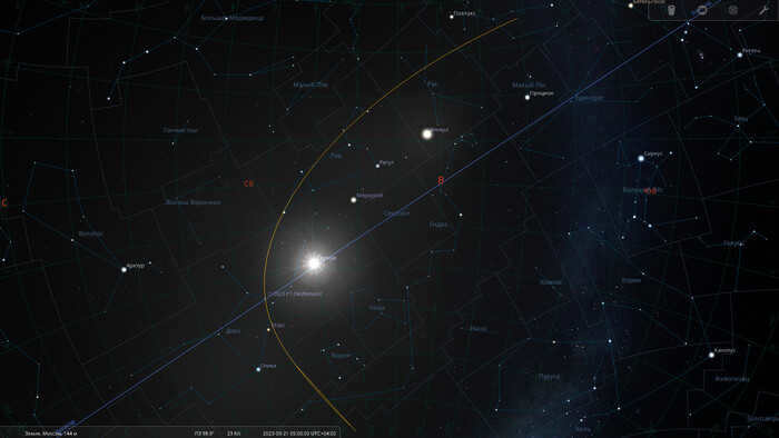
During perihelion, the comet is expected to have a brightness of approximately 2nd magnitude. In the evening sky of the northern hemisphere, the comet will be visible shortly after dusk, positioned in the northern part of the Virgo constellation. In the southern hemisphere, visibility of the comet will be either impossible or extremely challenging, as its declination is significantly higher than that of the Sun.
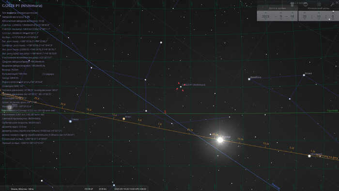
The comet C/2023 P1 will be located in the constellation Virgo on the evening of September 18, 2023, when it reaches its closest point to the Sun (perihelion).
As the days go by, the comet will gradually move further into the southern part of the sky, crossing the celestial equator around the same time as the Sun, just one day before the autumnal equinox on September 21, 2023. During this time, the comet’s brightness will diminish to a magnitude of 4.5.
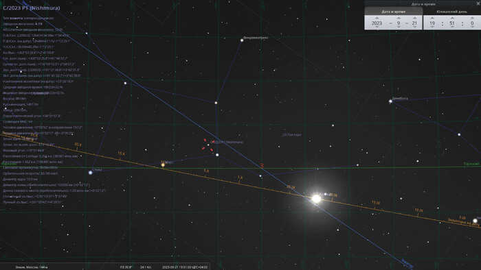
On the evening of September 21, 2023, you can find comet C/2023 P1 in the constellation Virgo
If you want to spot comet C/2023 P1 Nishimura on the evening of October 1, you’ll have to be in Australia or the mid-latitudes of South America… maybe at the southern tip of Africa. The comet’s brightness will only be about 7.5m, so it may not be worth buying tickets just for that.
On the evening of October 1, 2023, for an observer located in Cape Town, South Africa, comet C/2023 P1 can be seen at the boundary of the constellations Virgo and Raven.
By the middle of October, the comet will move even further south, appearing in the tail part of the constellation Hydra. Its brightness will decrease to the 10th magnitude, and visibility conditions, even in the southern hemisphere, will become unsatisfactory. Ultimately, at this point, the comet will no longer be visible to astronomy enthusiasts around the world.
When will the comet come back?
Not in our lifetime. Currently, the orbital elements have only been estimated. These estimations are sufficient to predict the comet’s position in the sky for the next few months, but we do not know the exact period of its orbit. Despite being categorized as a long-period comet, its eccentricity is believed to be equal to one, indicating that its orbit is nearly parabolic or possibly even is one. This means that the comet may return to the Sun in a million years or perhaps never.
The path of comet C/2023 P1 Nishimura from August 12 to November 1, 2023.
All visualizations were created using the Stellarium software.
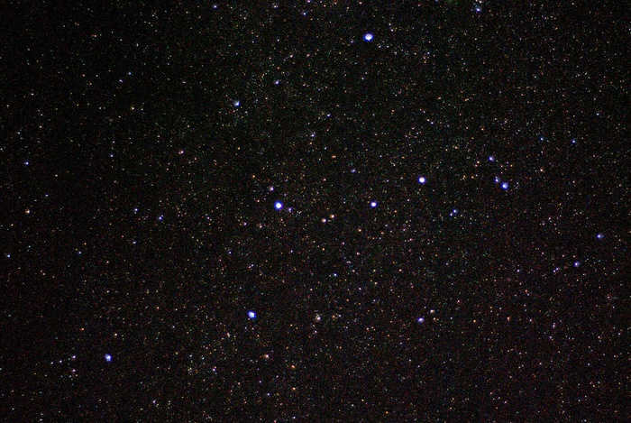
Orion’s Belt
The constellation Orion’s Belt is located 80 km from Minsk and was captured with a Nikon d80+ Nikkor 50mm 1.8 lens.
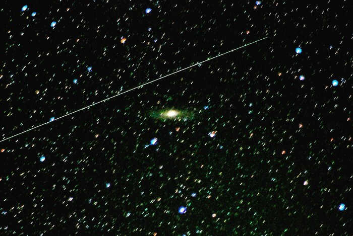
Andromeda Galaxy
I made my first attempt at capturing the Andromeda Galaxy through a telescope, but unfortunately, it didn’t go as planned. Despite using a 30-second exposure, a dark cloud obstructed my view, which left me frustrated. In the end, I decided to take a picture of the galaxy using a tripod and a 50 mm lens, and the results were much more satisfying. If anyone has experience with astrophotography through a telescope, I would greatly appreciate some advice on the correct technique. For your information, the telescope I used is a budget-friendly Celestron 70lt az.
The most irresistible properties in our solar system
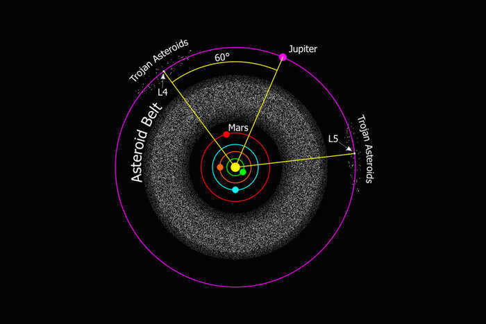
As we are all aware, the Soviet Union launched the first artificial satellite back in 1957. Since then, numerous space agencies, private companies, and research institutes have been expanding their presence in the solar system. The extent of their achievements is too numerous to list. While there seems to be ample space in this vast expanse for everyone, certain areas of local “real estate” are particularly enticing. One such example is the Lagrange points, which capture the attention of all interested parties. These points, named after an 18th-century mathematician who determined their location, offer unique stability in our constantly evolving corner of the cosmos.
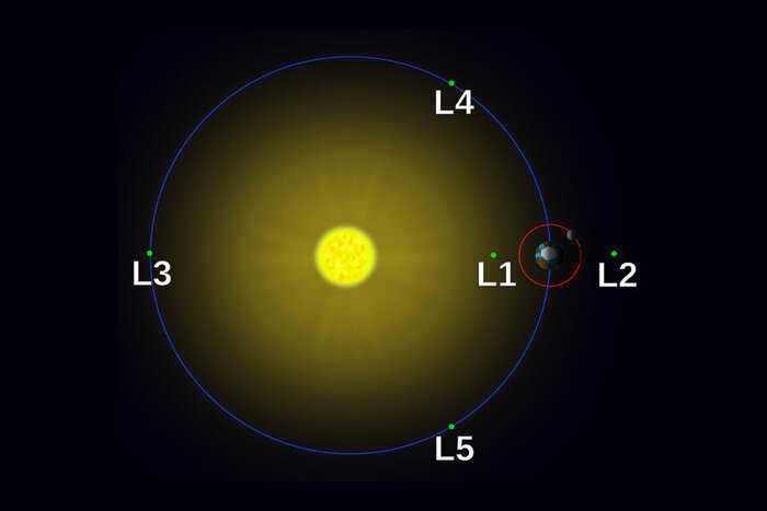
However, our system does not have many typical “parking lots”. The interaction of massive bodies creates five Lagrangian points for each pair of participants. For instance, the Sun has five points where it connects with any planet, and each planet has the same number of connections with its satellites. When you calculate it all, there are over 1000 Lagrangian points in our system, but only a handful of them are practically useful for human space exploration. Most of them are challenging to reach, and as we will discover later, not very stable. Currently, only two of these locations are actively utilized, but this circumstance might change in the future.
The issue of what can be placed in a specific Lagrangian point is quite intriguing. Let’s examine those created by the gravitational interaction between the Sun and Earth. L1 is positioned between these two celestial bodies, approximately 1.5 million kilometers from our planet. Because the line of sight to the star is never obstructed, it serves as an optimal location for observing the Sun.
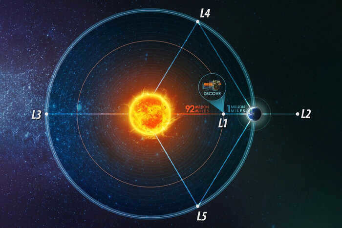
The Deep Space Climate Observatory is an American satellite designed to observe the Sun and Earth from Lagrangian point 1.
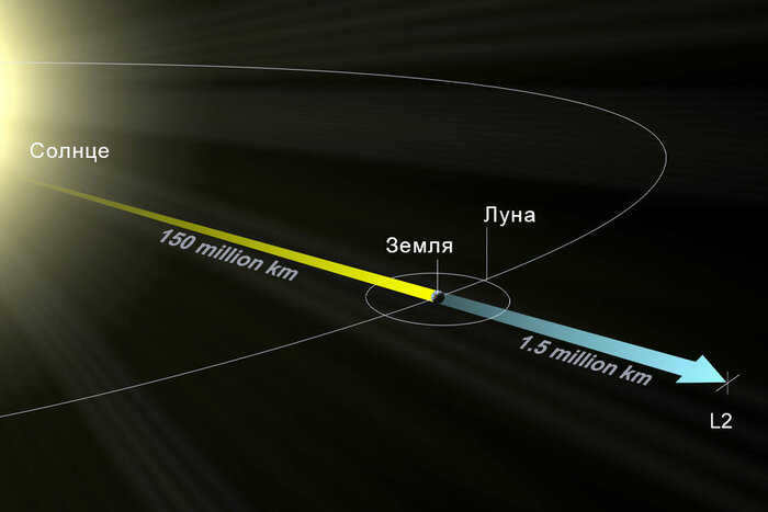
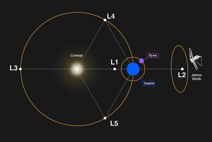
L2 is situated on the opposite side of the Earth at the same distance. This provides a safe shield from sunlight and offers unique opportunities for observing space in the opposite direction. In 2022, the long-awaited James Webb telescope began its operations from this location, a telescope that astronomers have been anticipating for two decades.
L3 is located in the most enigmatic region of the cosmos, precisely positioned on the opposite side of the Earth’s orbit in relation to the radiant Sun. This unique point in the vast universe is shrouded in mystery, as it remains completely hidden from the observation of any planet’s surface. Unsurprisingly, L3 has captivated the imaginations of numerous science fiction authors, who have delved into its potential wonders. However, from a scientific perspective, L3 offers limited utility and relevance.
L4 and L5 exhibit some differences compared to the previous Lagrangian points. The distinguishing factor is that the initial three points in each set of Lagrangian points possess a slight instability, causing objects within them to gradually shift sideways. While it is possible to maintain objects within these points if desired, it requires additional effort. In other combinations of celestial bodies, the stability of L4 and L5 might not be as high, particularly if their masses differ by less than a factor of 25. However, in the case of the Sun-Earth system, where the star significantly outweighs the planet, these points demonstrate remarkable stability. Additionally, they seem to attract various objects, with the most notable example being the L4 and L5 points of the Sun-Jupiter system, which have accumulated thousands of asteroids.
Each Lagrangian point within our solar system possesses its own unique characteristics. Some of these points could serve as ideal locations for gathering building materials, almost like drifting asteroids. Other points could potentially be utilized as refueling stations, providing a means to replenish fuel for spacecraft venturing into the depths of space. It’s even possible that human colonies could be established within these points, suspended in space. Naturally, this is a topic that pertains to the distant future, one that we may not witness ourselves, particularly given the current state of affairs on Earth. However, it’s always enjoyable to indulge in a bit of dreaming, isn’t it?
Thank you for taking the time to read this! If you enjoyed the article, you can show your support by giving it a “thumbs up” or subscribing to this channel. We would also like to inform you that we have our own Telegram channel where we regularly share fascinating posts about space and astronomy.
We truly value each and every one of our readers. If you would like to contribute financially (using the button below), your name/nickname will be acknowledged at the end of our next publication. This is our small way of expressing our gratitude for your generosity and support!
Double stars – observational characteristics: their definition along with pictures and videos, identification, categorization, multiples and variables, methods and locations for observing them in the constellation of Ursa Major.
Clusters of stars in the sky frequently arrange themselves in various formations, ranging from dense clusters to more dispersed ones. However, occasionally, there are stronger connections between individual stars. This is where we encounter binary systems, also known as double stars or multiples. In these systems, the stars have a direct impact on each other and progress in tandem. Notably, examples of such stars, even with the presence of variable stars, can be spotted within renowned constellations like the Big Dipper.
The exploration of binary stars
The exploration of binary stars was among the earliest accomplishments accomplished using astronomical binoculars. The initial arrangement of this kind was a duo Mizar in the constellation Ursa Major discovered by Riccioli, an Italian astronomer. Nonetheless, during that era, no data existed regarding whether there was a physical bond between the stars in such an arrangement.
Double stars, also known as binary stars, have been a topic of interest for many scientists. One theory suggests that these stars are formed from a common stellar association, based on their uneven brightness. This led some scientists to believe that these stars were separated by a significant distance, making it impossible for them to be connected. To test this hypothesis, the annual stellar parallax needed to be measured.
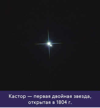
In 1804, William Herschel, who had been observing for 24 years, released a catalogue documenting 700 double stars. This catalogue contained information on 700 double stars. Herschel addressed the contradiction of the hypothesis and attempted to resolve it. To his surprise, he discovered that each star followed a complex elliptical trajectory, rather than a symmetrical oscillation with a six-month period, as previously believed.
Based on the principles of celestial mechanics, two bodies that are gravitationally bound will move in an elliptical orbit. Therefore, Herschel’s findings provided evidence supporting the assumption that there is a gravitational connection in double star systems.
Binary systems are also classified by their observational characteristics:
Visually observable binary stars
Binary stars that can be distinguished as separate entities (or are said to be capable of being resolved) are referred to as
visually observable binaries
or
visual binaries
.
The ability to perceive a star as a visual pair depends on the resolving power of the telescope, the distance to the stars, and the separation between them. Thus, visually double stars are primarily those located close to the Sun, with extremely long orbital periods resulting from the significant distance between the star components. Due to these extended periods, the orbit of a double star can only be determined through numerous observations spanning several decades.
Currently, the WDS and CCDM catalogs contain more than 78,000 and 110,000 objects respectively, but only a few hundred of them have orbits that can be calculated. For less than one hundred of these objects, the orbit is known with enough precision to determine the masses of the components.
When observing a visual double star, we measure the separation between the components and the angle at which the line connecting the two stars is oriented in relation to the north pole of the world.
Double stars observed using speckle interferometry
Speckle interferometry, combined with adaptive optics, enables us to achieve the maximum resolution possible for stellar observations. This enhanced resolution allows us to detect double stars.
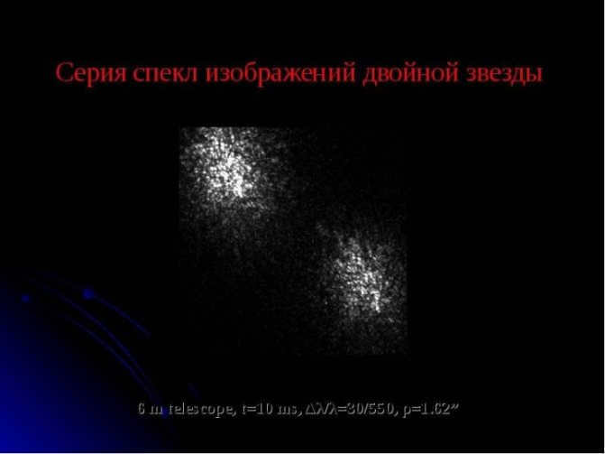
In essence, speckle interferometric doubles can be considered equivalent to visual doubles. However, unlike the classical visual-double method which requires obtaining two distinct images, speckle interferograms are analyzed in this case.
Speckle interferometry proves to be efficient when studying doubles with periods spanning several decades.
When it comes to visual binary stars, we observe the simultaneous motion of two objects across the celestial sphere. Nevertheless, if we hypothesize that one of the two components is imperceptible to us due to various factors, we can still identify the duality by noting the alteration in the position of the second object in the sky. In such instances, these stars are referred to as astrometric binary stars.
If high-precision measurements of the positions of stars are available, the concept of duality can be inferred by determining the nonlinearity of their motion, specifically their first and second derivatives. Astrometric binary stars are utilized to determine the masses of brown dwarfs belonging to various spectral classes.
Observing Spectral Double Stars
Spectral double stars are stars that exhibit duality when observed through spectral analysis. To detect this duality, astronomers observe the star over multiple nights. If they notice periodic shifts in the lines of the star’s spectrum, it indicates a change in the star’s velocity.
There are various reasons for these shifts, such as the star’s own variability or the presence of an expanding shell resulting from a supernova explosion.
If the spectrum of the second star component is obtained and shows similar shifts, but in the opposite phase, then astronomers can confidently conclude that they are observing a double star system. When the first star is approaching and its spectral lines are shifting towards the violet side of the spectrum, the second star is moving away and its lines are shifting towards the red side, and vice versa.
However, if the brightness of the second star is significantly lower than that of the first, there is a chance that we may not be able to see it. In such cases, we need to consider other possible options. The key characteristic of a double star is the periodic variation of radial velocities and the significant difference between the maximum and minimum velocities. Nevertheless, it is not entirely impossible for an exoplanet to exist alongside a double star.
In addition to determining the masses of the components, spectroscopic data can also be used to calculate the distance between them, the orbital period, and eccentricity. However, these data cannot provide information about the angle of inclination of the orbit with respect to the line of sight. Therefore, it is only possible to speak of the mass and distance between the components with accuracy up to the angle of inclination, as calculated.
When it comes to any celestial objects that astronomers study, there are collections of double stars with different spectra. The most famous and comprehensive catalog is called “SB9” (which stands for Spectral Binaries). Currently, it includes 2839 objects.
Eclipsing double stars.
There are instances where the orbital plane is inclined at a very small angle to the line of sight: the orbits of stars in such a system are positioned in a way that they appear as if they are edges to us. In such a system, the stars will go through periodic eclipses, meaning the brightness of the pair will fluctuate. These double stars with eclipses are known as eclipsing-doubles or eclipsing-variable stars.
The most well-known and initially discovered star of this kind is Algol (also known as Devil’s Eye) in the Perseus constellation.
Doubles in the Microlensing Phenomenon
Microlensing is utilized to detect double stars where both components consist of low-mass brown dwarfs.
If there is a celestial object with a significant gravitational field situated along the line of sight between the star and the observer, the object will act as a lens. If the gravitational field were powerful enough, multiple images of the star would be visible. However, in the case of galactic objects, their gravitational field is not strong enough for the observer to discern multiple images. This is referred to as microlensing.
When the gravitating body is a binary star system, the resulting light curve obtained from its passage across the observer’s line of sight is markedly distinct from that of a single star.
Light curves
Here are some examples of light curves for a split double system:
Take a look at these light curves for a close double system:
If the double star is an eclipsing star, it is possible to plot the time dependence of the integral light. The variability of the light on this curve will depend on the following factors:
- The eclipses themselves
- The effects of ellipsoidality
- The effects of reflection, or rather recycling, of radiation from one star in the atmosphere of another
However, when analyzing only the eclipses themselves, assuming the components are spherically symmetric and there are no reflection effects, we can reduce the problem to solving the following system of equations:
where ξ, ρ represent polar distances on the disk of the initial and subsequent stars, Ia denotes the absorption function of radiation from one star through the atmosphere of the other, Ic denotes the brightness function of the dσ sites of various components, Δ represents the overlapping region, and rξc and rρc are the overall radii of the initial and subsequent stars.
It is not feasible to solve this system without any prior assumptions. Similarly, it is not possible to analyze more complex scenarios involving ellipsoidal-shaped components and reflection effects, both of which are significant in different variations of close binary systems. As a result, all contemporary methods of light curve analysis inevitably incorporate model assumptions, with parameters determined through other types of observations.
Radial velocity curves
When observing a double star spectroscopically, which means it is a spectroscopic double star, it becomes possible to create a graph showing the change in radial velocities of the components over time. Assuming the orbit is circular, the following equation can be written:
where Vs represents the radial velocity of the component, i is the inclination of the orbit to the line of sight, P is the period, and a is the radius of the component’s orbit. If we substitute Kepler’s third law into this equation, we get:
Where Ms is the mass of the component being studied, and M2 is the mass of the second component. By observing both components, we can determine the ratio of the masses of the stars that make up the double star. By applying Kepler’s third law again, we can simplify the equation to:
where G is the gravitational constant and f(M2) is a function of the star’s masses and is defined as:
In the scenario where the orbit is not circular but instead has eccentricity, it can be proven that the mass function must be dominated by the factor in order to determine the orbital period P.
If the second component of the system is not observed, the function f(M2) provides a lower limit on its mass.
It is important to note that by solely studying the radial velocity curves, it is impossible to determine all the parameters of the binary system. There will always be uncertainty in the form of an unknown orbital inclination angle.
Determining the masses of the components
In most cases, the gravitational interaction between two stars can be adequately described using Newton’s laws and Kepler’s laws, which are derived from Newton’s laws. However, in the case of double pulsars, general relativity (GR) must be taken into account. By studying the observable effects of relativistic phenomena, we can once again verify the accuracy of the theory of relativity.
Kepler’s third law establishes a relationship between the rotation period, the distance between the components, and the mass of the system:
Whereas in a visual-double system it is possible to calculate the period, semi-major axis, and mass ratio by determining the orbits of both components, this duality can often only be inferred from spectral data in a spectral-double system. By analyzing the motion of spectral lines, it is possible to determine the radial velocities of one or both components. If only the radial velocity of one component is known, it is not possible to obtain complete information about the masses. However, a mass function can be constructed, allowing for the determination of an upper limit on the mass of the second component. This information can help determine whether the second component could be a black hole or a neutron star.
a Centauri
can be paraphrased as “Alpha Centauri”.
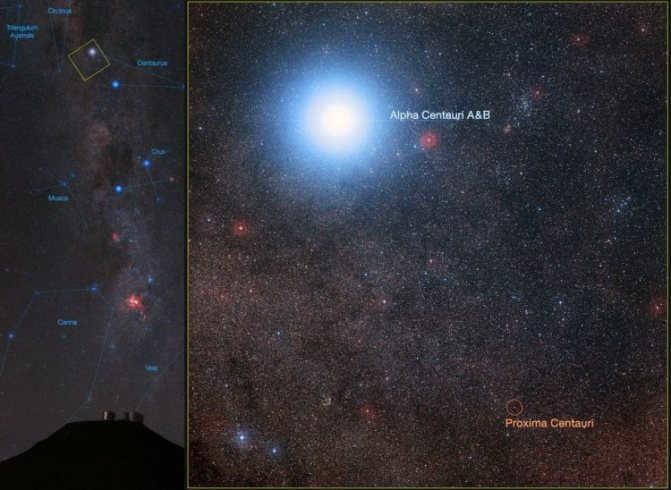
a Centauri consists of two stars – a Centauri A and a Centauri B:
a Centauri A has similar parameters to the Sun: Spectral Class G, a temperature of approximately 6000 K, and the same mass and density;
a Centauri B has a mass 15% lower, spectral class K5, temperature 4000 K, diameter 3/4 that of the Sun, and an eccentricity (the degree of elongation of an ellipse equal to the ratio of the distance from the focus to the center to the length of the major semi-major axis, i.e. the eccentricity of a circle is 0 – 0.51).
The period of revolution is 78.8 years, the average distance from the sun is 23.3 astronomical units, the orbital plane is tilted at an angle of 11 degrees relative to the line of sight, the center of mass of the system is moving towards us at a velocity of 22 km/s, the transverse velocity is 23 km/s, meaning the total velocity is directed towards us at an angle of 45 degrees and has a magnitude of 31 km/s.
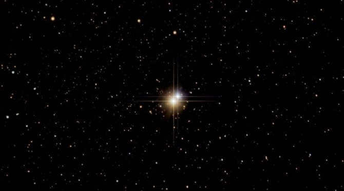
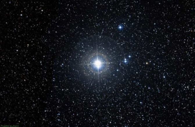
Sirius: The Brightest Star in the Night Sky
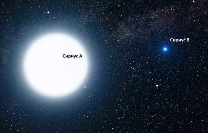
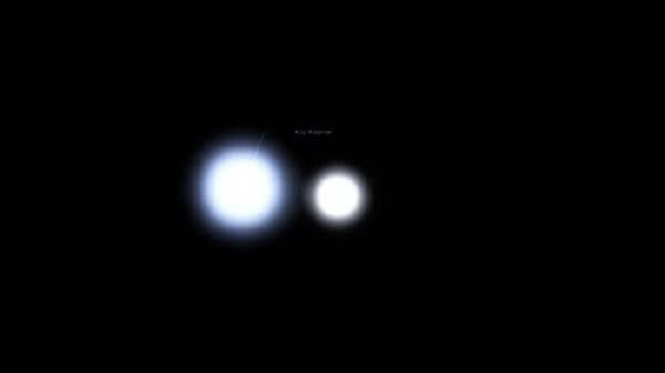
Sirius, similar to Centauri, is composed of two stars – A and B. However, unlike Centauri, both stars in Sirius have spectral class A (A-A0, B-A7) and, as a result, a significantly higher temperature (A-10000 K, B-8000 K).
The mass of Sirius A is 2.5 times that of the sun, while Sirius B is 0.96 times the mass of the sun. As a result, both stars emit the same amount of energy from their surfaces, but the satellite is 10,000 times less luminous than Sirius. Therefore, its radius is 100 times smaller, making it almost the same size as Earth. Despite this, it has a mass almost equal to that of the Sun, resulting in a high density for the white dwarf.
During the study of Sirius, the presence of the satellite went unnoticed for a significant period of time due to its exceptionally high density, which is 75,000 times greater than that of Sirius A. As a result, the satellite’s size and luminosity are approximately 10,000 times smaller.
Notes
- ↑ 12A.A. Kiselev.
Double stars
(unpublished)
. Astronet (12.12.2005). Date of circulation April 27, 2013. - ↑ 12345А. V. Zasov, K. A. Postnov.
General astrophysics. – Fryazino: VEK 2, 2006. – С. 208-223. – 398 с. – 1500 copies. – ISBN 5-85099-169-7. - Speckle Interferometry and Orbits of “Fast” Visual Binaries
- V. V. Makarov and G. H. Kaplan.
Statistical Constraints for Astrometric Binaries with Nonlinear Motion. — Bibcode: 2005AJ….129.2420M. - Pope, Benjamin; Martinache, Frantz; Tuthill, Peter.
Dancing in the Dark: New Brown Dwarf Binaries from Kernel Phase Interferometry. — 2013. — Bibcode: 2013ApJ…767..110P. - Gravitational Microlensing of Binary Stars: Light Curve Synthesis. — 1997. (unavailable link)
- Choi, J.-Y.; Han, C.; Udalski, A.; Sumi, T etc.
Microlensing Discovery of a Population of Very Tight, Very Low Mass Binary Brown Dwarfs. — 2013. — Bibcode: 2013ApJ…768..129C. - V.M. Lipunov.
Algol Paradox
(not available)
. - Richard B.Larson.
Implications of binary properties for theories of star formation (English). — 2001. Archived on May 28, 2008. - ↑ 123Kaitlin M. Kratter.
The creation of binary star systems (English). — 2011. — Bibcode: 2011ASPC..447…47K. — arXiv:1109.3740. - ↑ 123Zhou, Ji-Lin; Xie, Ji-Wei; Liu, Hui-Gen; Zhang, Hui; Sun, Yi-Sui.
The process of forming various planetary systems. - ↑ 123А. В. Goncharskii, A.M. Cherepashchuk, A.G. Yagola.
Unresolved issues in astrophysics. – Moscow: Nauka, 1985. – P. 68-101. – 351 p. – 2500 copies. - Hans Zinnecker.
Historical milestones of binary stars (in English): conference proceedings. – The formation of binary stars IAU symposium, 2001. – Vol. 200. Archived May 28, 2008.
Double Stars and their Planetary Systems
The exploration of planetary systems in double stars commenced during the 1980s, predating the discovery of the initial indications of exoplanets, which are planets located beyond our own solar system.
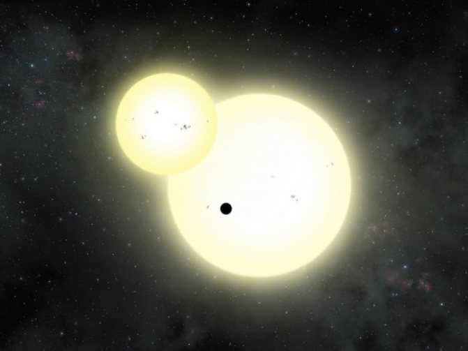
While the passages in a binary star system may appear more complex, the possibility of discovering such planets was inspired by a basic assumption: if a planet does orbit a binary star system, it is likely to follow the same orbital plane as the stars themselves.
In simpler terms, if, from the perspective of an observer on Earth, the stars eclipse each other, then it is probable that the planet will cast a shadow on one or both stars.
It is estimated that out of all the exoplanets identified so far, approximately a hundred orbit around binary star systems.
One cannot forget the iconic planet Tatooine from the Star Wars movie, which serves as Luke Skywalker’s home planet. Due to its orbit around two stars, it appears as a parched, sandy world.
In the real world, thanks to observatories such as the Kepler Space Telescope, we are aware that a binary star system has the potential to have exoplanets.
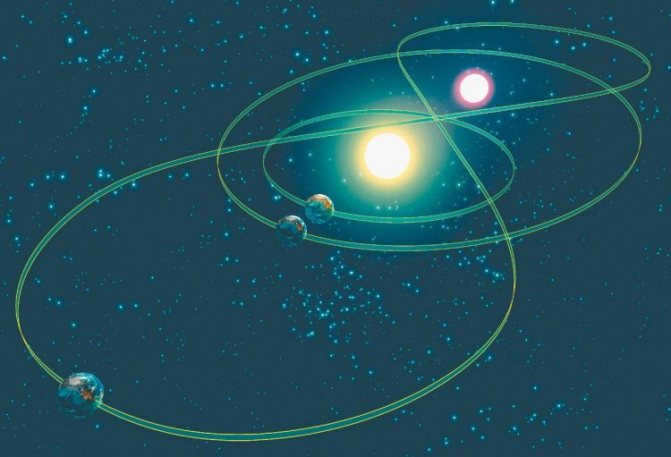
The orbits of planets in binary star systems
Scientists specializing in planetary research have also made the discovery that such a celestial body can be quite habitable, given that it is situated at an optimal distance from its two stars. Furthermore, it is not necessary for it to be completely uninhabited. According to a recent investigation, within a specific range of distances from two stars resembling our sun, there may exist a planet with liquid water, capable of maintaining both water and suitable living conditions for extended periods of time.
Discover the Beauty of Double Stars with Binoculars
When it comes to exploring the night sky, a pair of high-quality astronomical binoculars is an invaluable tool. One of the key advantages they offer over telescopes is their ability to provide a wide field of view. Unlike telescopes, which may struggle to fit certain objects entirely within the eyepiece or lose their visual impact when they occupy the entire field of view, binoculars allow for a more immersive and breathtaking experience.
Within the vast expanse of the night sky, there are countless double and variable stars waiting to be discovered with binoculars. These celestial gems offer stunning beauty against the backdrop of the Milky Way, and their splendor can truly be appreciated by those wielding wide-angle instruments. Here, we present a selection of some of the most mesmerizing double stars that can be observed with binoculars:
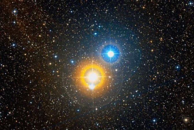
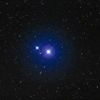
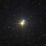
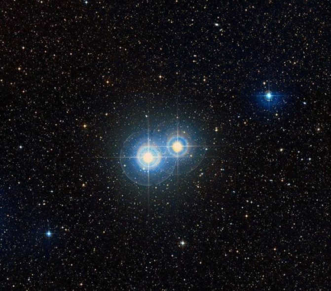
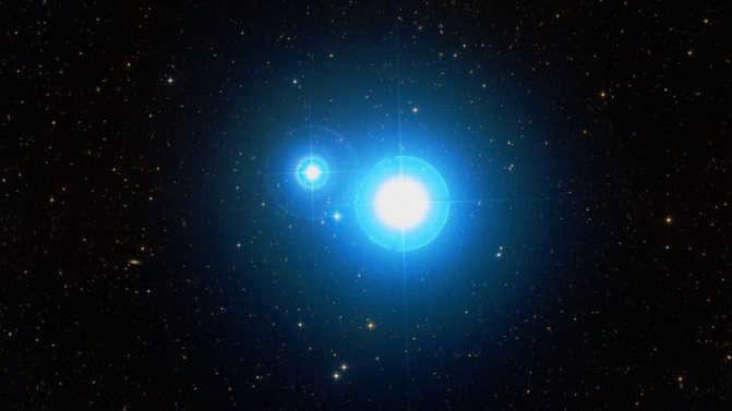
Albireo (also known as the Swan’s β) is renowned for being one of the most prominent binary stars in the night sky. Albireo can be effortlessly located as it serves as the head of a bird within the constellation of the Swan. Even with binoculars as small as 30mm, one can discern the individual components of Albireo, and the striking color contrast between the two components never fails to captivate seasoned stargazers. The visual appeal of Albireo is so remarkable that it even translates well in photographs, which often struggle to accurately capture the true colors of stars. Needless to say, the experience of observing Albireo firsthand is truly awe-inspiring!
The primary element of the system is characterized by a vibrant yellow hue, bordering on orange. Renowned stellar nomenclature researcher Richard Allen aptly described the color of this celestial body as “topaz yellow.” Its luminosity registers at approximately 3 on the star magnitude scale. Positioned at a distance of 34″ from the main star, a bluish-white companion shines with a brilliance of 5m. The stark contrast between the two stars accentuates the blue star’s vibrant hue, making it appear even bluer than other hot stars, including Vega!
Albireo is observable during the summer and fall evenings, as well as in the spring mornings.
The Leader of the Hound Dogs
The Hound Dog’s Alpha, also known as the Heart of Charles II, can be found just below the handle of the Big Dipper in the sky. It is easily visible at almost any time of year, except in late summer and early fall when it is positioned very low on the horizon. The two components in this pair are closer together than the Albireo components, being at a distance of 20″. The host star has a bluish color, while its companion is yellow.
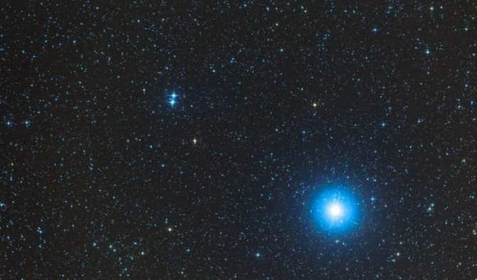
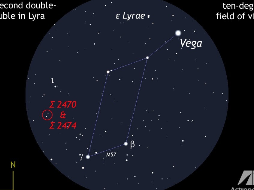
This double star is widely known as one of the most famous in the entire sky, and it is particularly popular among astronomers observing the constellation Lyra. It is consistently mentioned in all reference books and guidebooks, highlighting its significance. With a distance of 208″ between its components, this pair is easily distinguishable in binoculars, and some individuals with exceptional visual acuity can even spot it with the naked eye. The presence of the stunning stellar background and the nearby star Vega further enhances the appeal of observing this star, making it a must-see for any astronomy enthusiast with binoculars!
The Lyra Delta
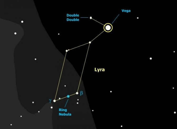
In the constellation Lyra, there is another wide double star known as δ Lyrae. This star, also called Lyra delta, is located at the upper left corner of the parallelogram just below Vega.
The main star in this double system appears red in color, while its companion has a bluish-white hue. The two stars are not physically connected but appear close together at a separation of 619″ or 10 arc minutes. This is an optical pairing, where the stars only appear to be aligned in the same direction. What makes this double star special is its surroundings: the bright stars of Lyra, with the stunning Vega leading the way, create a beautiful celestial scene!
To observe Lyra delta, as well as the other double stars in the constellation Lyra mentioned below, the best times are spring mornings, summer nights, and fall evenings.
Mizar and Alcor
Mizar and Alcor are two stars in the Big Dipper constellation. They are often referred to as a binary star system because they appear close together in the sky. Mizar is the brighter of the two stars, while Alcor is slightly dimmer. Despite their proximity, Mizar and Alcor are not physically connected and are actually located at different distances from Earth. They have been a popular target for stargazers throughout history and have even been used as a test of visual acuity. In fact, the ability to see both Mizar and Alcor with the naked eye is often considered a measure of good eyesight.
Maybe we should have begun with this pair of stars, as it is the most well-known double in the whole night sky! Mizar and Alcor are separated by a distance of 12 angular minutes in the sky and are easily visible individually to the naked eye.
Through powerful binoculars, it becomes apparent that Mizar itself is a binary star. Additionally, several other stars can be observed between Mizar and Alcor using binoculars, with the brightest star even having its own designation, the Star of Louis. All of these stars, including the Star of Ludovico, serve as a backdrop, enhancing the brilliance of the bright white components of Mizar and the equally white Alcor.
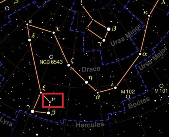
In the constellation of Draco, there is a group of stars known as the Dragon’s Head, with the star ν often referred to as the “eyes of the Dragon”. This asterism is positioned above the star Vega and forms an irregular quadrangle with stars of 2nd and 3rd magnitudes. The dimmest star in this quadrangle is ν of the Dragon.
Within this star, there are two stars of equal brightness separated by 1 arc minute. Under ideal conditions, individuals with exceptional eyesight may be able to perceive these stars separately with the naked eye. However, this requires venturing far away from urban areas and observing on a night that is exceptionally dark and clear.
The two white stars of spectral class A in the ν Dragon system are almost identical, resembling each other closely. They are separated by a distance of at least 1900 astronomical units (a.u.) and orbit around a common center of mass. It takes them approximately 44,000 years to complete one revolution.
Delta Cepheus
Not many individuals are aware that the renowned variable star, delta Cepheus, which has served as the prototype for an entire class of Cepheid variable stars, possesses a companion star within its vicinity. This companion star, a pale blue celestial body with a luminosity of 6.3m, is situated at a distance of 41″ from the main star. In terms of appearance, the pair bears a resemblance to Albireo, although the contrast between the components is not as pronounced (Cepheus’ δ is a pale yellow).
One of the advantages of Delta Cepheus is that it can be observed throughout the year in Russia and neighboring countries.
Engaging trivia
- Around 50% of the stars in the observable Universe exist in pairs, known as double stars. It is possible that there are even more double stars than single stars.
- In most cases, both companions in a double star system are of the same age, but one of them may have a higher mass and be at a different stage of evolutionary development.
- Occasionally, double star systems can contain neutron stars or black holes.
- Double stars have the ability to exchange matter with each other.
- Amateur astronomers make a distinction between optically double and physically double star systems. Optically double stars are simply stars that appear side by side in the night sky, while physically double stars are true double star systems where both companions orbit a common center of mass.
Greater Multiples
Researchers are aware of star systems with a higher number of components as well. Consequently, Scorpius consists of more than seven celestial bodies.
Consequently, it has been revealed that star systems in the galaxy, as well as the planets within them, are not identical. Each one possesses its own distinctiveness, variation, and highly captivating nature. Researchers continue to unearth an increasing number of stars, and it is possible that in the near future, we will acquire knowledge about the existence of sentient life beyond the confines of our own planet.
A binary system, also known as a double star, consists of two stars that are gravitationally bound and orbit around a common center of mass. Double stars play a crucial role in determining the masses of stars and establishing various relationships. The mass-radius, mass-luminosity, and mass-spectral class relationships are essential in understanding the internal structure and evolution of stars.
The significance of double stars extends beyond just providing mass information. For instance, all black hole candidates discovered so far have been found in double systems, despite numerous attempts to find single black holes. Additionally, Wolf-Rayet stars have been extensively studied due to their association with double stars.
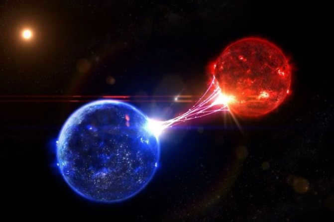
Gravitational interaction between the components
Types of binary stars and how they are detected
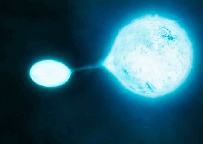
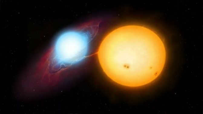
An illustration of a compact binary system. The image shows the Variable star Mira (omicron Keith) captured by the Hubble Space Telescope in ultraviolet light. The photo reveals a stream of material flowing from the primary component, a red giant, to the companion, a white dwarf
Physically, binary stars can be classified into two groups:
- stars that have experienced, are experiencing, or will experience mass transfer – close binary systems,
- stars that cannot exchange mass – wide binary systems..
If we classify binary systems based on the mode of observation, we can identify visual, spectral, eclipsing, astrometric double systems.
Visual binary stars
Binary stars that can be observed as separate entities (or are said to be capable of being resolved) are referred to as visible binaries or visual binaries.
Spectral binary stars
A spectral binary refers to a binary star system where the presence of two stars can be detected through spectral observations. In order to determine if a star system is a spectral binary, astronomers observe the star over multiple nights and analyze the behavior of its spectral lines. If the wavelengths of the spectral lines vary from night to night, it indicates that the velocity of the source is changing. There can be various factors causing this, such as the variability of the star itself or the presence of an expanding shell resulting from a supernova event. By comparing the spectral behavior of the first star with that of the second star, it is possible to confirm the presence of a double star system. It is important to note that if the first star is moving towards us, its spectral lines will shift towards the violet end of the spectrum, while the second star will move away from us, causing its lines to shift towards the red end of the spectrum, and vice versa.
However, if the brightness of the second star is significantly lower than that of the first, there is a possibility that we may not be able to see it. In such cases, we need to consider all possible scenarios. The primary evidence supporting the existence of a double star system is the periodic variation in radial velocities and the significant difference between the maximum and minimum velocities. However, if we carefully analyze these arguments, we can also make a case for the discovery of an exoplanet. To address any uncertainties, it is crucial to calculate the mass function. This calculation can provide insights into the minimum mass of the second component and help determine whether the invisible object is a planet, a star, or even a black hole.
Additionally, spectroscopic data allows for the calculation of various parameters such as the mass and distance between components, as well as the period of rotation and eccentricity of the orbit. However, the angle of inclination to the picture plane cannot be directly observed. Therefore, when discussing the mass and distance between components, it is necessary to take into account the calculated values with consideration to the inclination angle.
Similar to other objects studied by astronomers, there are catalogs specifically dedicated to spectral double stars. One of the most well-known and comprehensive catalogs is SB9, which currently includes 2839 objects.
It occasionally occurs that the orbital plane intersects or nearly intersects the line of sight of the observer. The stars in such a system follow orbits that appear, in a sense, ribbed to us. In this scenario, the stars will periodically pass in front of each other, resulting in a change in brightness for the entire pair at regular intervals. This specific kind of binary system is referred to as an eclipsing binary. When discussing the variability of the star, it is then classified as an eclipse-variable star, which also highlights its dual nature. The first and most well-known example of this type of binary is the star Algol (also known as the Devil’s Eye) located in the constellation Perseus.
Astrometric double stars: an insight into the hidden universe
Occasionally, in the vast expanse of space, celestial bodies come together in a unique and fascinating way. Astrometric double stars, as they are called, are a result of one star being either incredibly small or possessing a low luminosity. These elusive stars cannot be seen directly, but their presence can be inferred through careful observation.
When a star is part of an astrometric double system, the brighter component will occasionally deviate from its expected trajectory. It will seemingly wander off course, moving to one side or the other. This peculiar behavior can be explained by the motion of the system’s center of mass. The magnitude of these deviations is directly proportional to the mass of the unseen star.
Take, for example, Ross 614, one of the closest stars to our own. Studies have revealed that this star exhibits a significant 0.36″ deviation from its predicted path. This astonishing revelation has shed light on the intricacies of this hidden universe. Furthermore, it has been determined that Ross 614 completes a full orbit around its unseen companion every 16.5 years.
As our understanding of the universe deepens, astronomers have discovered approximately 20 astrometric double stars in close proximity to our own Sun. Each of these systems provides a unique opportunity to explore the mysteries of the cosmos and unravel the secrets of the unseen.
Components of binary stars
There are various types of binary stars: some consist of two similar stars, while others have different characteristics. However, regardless of their nature, binary stars provide excellent opportunities for study. Unlike ordinary stars, their interactions can reveal valuable information about their mass, orbital shape, and even provide insight into neighboring stars. Mutual attraction causes these stars to have a slightly elongated shape. Approximately half of the stars in our Galaxy are part of binary systems, making binary stars a common occurrence.
Being part of a binary system significantly impacts the life of a star, especially when the companions are in close proximity. The exchange of matter between the stars can lead to dramatic events, such as the eruption of novae and supernovae.
The likelihood of planets existing in star systems with two or three stars has always been seen as extremely unlikely. However, a planet in such a system has recently been found ([1]).
For further information
Sources
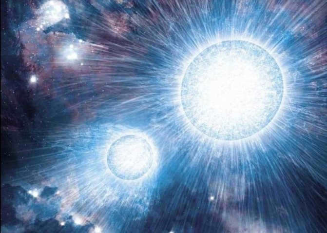
An artist’s interpretation of a binary system consisting of O stars
A double star, also known as a double system, is a celestial system comprising two stars that are gravitationally bound and revolve around a shared center of mass. Double stars are a prevalent phenomenon, with approximately half of all stars in our Milky Way galaxy existing in binary systems. By studying the orbital period and the distance between these stars, scientists can sometimes calculate the masses of the individual components. This approach requires minimal additional assumptions and is thus a primary method for determining masses in the field of astrophysics. Consequently, double systems containing black holes or neutron stars are of significant interest to the astrophysics community.
Classification
- Stars that cannot exchange mass in principle are called separated binary systems.
- Stars that have, will have, or have had an exchange of mass are called close binary systems. These can be further divided into:
- Semi-separated, where only one star fills its Roche cavity.
- Contact, where both stars fill their Roche cavities.
Binary systems can also be classified based on the method of observation. We can distinguish visual, spectral, eclipsed, and astrometric double systems.
Visually observable binary stars
Binary stars that can be observed separately (or are claimed to be resolvable) are referred to as visually observable binaries or visual binaries.
When observing a visual binary star, astronomers measure both the separation between the two components and the positional angle of the line connecting them. The positional angle is the angle between the direction towards the north pole and the direction of the line connecting the primary star and its companion.
Double stars detected through speckle-interferometric techniques
Speckle interferometry, in combination with adaptive optics, enables astronomers to achieve the diffraction limit of stellar resolution, allowing them to identify double stars. Essentially, speckle-interferometric doubles are equivalent to visual doubles. However, unlike the traditional visual-double method that requires obtaining two separate images, speckle interferometry involves analyzing speckle-interferograms.
Speckle interferometry proves particularly effective in detecting double stars with orbital periods lasting several decades.
Astrometric binary stars
The behavior of an astrometric binary star system in the night sky.
In the scenario of visual binary stars, we observe two celestial objects moving across the sky in tandem. However, if one of the two components is not visible to us for any given reason, the duality can still be detected by observing the change in position of the remaining component in the sky. In such cases, we refer to these systems as astrometric binary stars.
By utilizing high-precision astrometric observations, the duality can be inferred by tracking the nonlinearity of motion, both in terms of its first derivative and its second derivative. Astrometric binary stars are particularly useful in measuring the masses of brown dwarfs belonging to different spectral classes.
An example of bifurcation and line shifting in the spectra of spectrally double stars can be observed under certain conditions.
A spectrally double star refers to a star that exhibits duality based on spectral observations. In order to determine this, the star is observed over multiple nights. If it is found that the lines in its spectrum shift periodically over time, it indicates a change in the velocity of the source. There can be several factors contributing to this phenomenon, such as the variable nature of the star itself or the presence of a dense expanding shell resulting from a supernova eruption, among others.
If we observe the spectrum of the second component and notice similar displacements, but in opposite phase, then we can conclude that we are dealing with a binary system. In the case where the first star is moving towards us and its spectral lines are shifted towards the violet side, while the second star is moving away and its lines are shifted towards the red side, we can confidently determine the presence of a double system. The opposite scenario also holds true.
However, if the brightness of the second star is significantly lower than that of the first star, there is a possibility that we may not be able to observe it. In such cases, we must explore other potential options. The key indicator of a binary star system is the regularity of changes in radial velocities and the substantial disparity between the maximum and minimum velocities. Nevertheless, it is technically not impossible for an exoplanet to have been detected. To determine this, we must calculate the mass function, which allows us to estimate the minimum mass of the unseen second component and thus determine whether it is a planet, a star, or even a black hole.
Moreover, by analyzing spectroscopic data, we can not only determine the masses of the components, but also calculate various other parameters such as the distance between them, the orbital period, and the eccentricity. However, it is important to note that these data alone cannot provide information about the angle of inclination of the orbit to the line of sight. Therefore, when discussing the mass and distance between the components, we can only speak of them as calculated with precision up to the angle of inclination.
Like any other type of celestial objects studied by astronomers, spectrally double stars have their own catalogs. One of the most well-known and comprehensive catalogs is the “SB9” catalog, which stands for Spectral Binaries. Currently, it boasts a collection of 2839 objects.
Eclipsing binary stars
In certain cases, the orbital plane of a binary star system is inclined at a very slight angle to our line of sight, causing the stars’ orbits to appear edge-on to us. When this happens, the stars will periodically pass in front of each other, resulting in variations in their brightness. These types of double stars are known as eclipsing binaries or eclipsing variable stars. One of the most well-known and first discovered stars of this kind is Algol (also known as the Devil’s Eye) in the constellation Perseus.
If a body with a powerful gravitational field is positioned directly between the star and the observer, the object will undergo lensing. If the gravitational field is sufficiently strong, multiple images of the star will be visible. However, with galactic objects, the field is not strong enough for the observer to discern multiple images. This phenomenon is known as microlensing. When the gravitating body is a binary star system, the resulting light curve observed differs significantly from that of a single star.
Microlensing is a technique utilized to search for binary stars in which both components are low-mass brown dwarfs.
Phenomena and occurrences related to binary stars
The Algol enigma
This enigma was formulated during the mid-20th century by Soviet astronomers A. G. Masevich and P. P. Parenago, who noticed a discrepancy between the masses of the Algol components and their stage of evolution. According to the theory of stellar evolution, a massive star evolves at a much faster rate than a star with a mass similar to or slightly larger than the Sun. It is logical to assume that the components of a binary star system formed at the same time, indicating that the more massive component should have evolved sooner than the lower-mass component. However, in the Algol system, the more massive component was actually younger.
The resolution of this paradox is connected to the occurrence of mass transfer in close binary systems and was initially suggested by American astrophysicist D. Crawford. If we hypothesize that one of the components has the ability to transfer mass to its companion during evolution, the paradox is resolved.
Interstellar Mass Transfer
Representation of equipotential surfaces in the orbital plane of a binary system according to the Roche model
- It is assumed that the stars are concentrated masses and their intrinsic angular momentum can be disregarded in comparison to their orbital angular momentum.
- The components rotate in perfect synchronization.
- The orbit is perfectly circular.
where r1= √x 2 +y 2 +z 2 , r2= √(x-a) 2 +y 2 +z 2 , μ = M2/(M1+M2) , and ω is the orbital rotation frequency of the components. By utilizing Kepler’s third law, the Roche potential can be rephrased as:
where the dimensionless potential is:
Equipotentials are derived from the equation Φ(x,y,z)=const . In close proximity to the centers of the stars, they bear little difference from the spherical ones, but as we move away, the deviation from spherical symmetry becomes more pronounced. Ultimately, both surfaces converge at the Lagrangian point L1 . This implies that the potential barrier at this point is 0, enabling particles from the star’s surface near this point to enter the Roche cavity of the adjacent star, thanks to thermal chaotic motion.
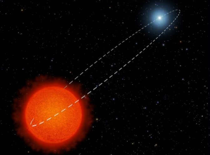
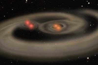
Symbiotic Stars: A Unique Phenomenon in the Universe
Symbiotic stars are extraordinary double systems consisting of a red giant and a white dwarf, encircled by a captivating common nebula. These celestial objects exhibit complex spectra, showcasing a fascinating blend of absorption bands, such as TiO, and emission lines that are characteristic of nebulae, such as OIII and NeIII.
One of the distinguishing features of symbiotic stars is their variability, with periodic fluctuations spanning several hundred days. These enigmatic stars also undergo new-like outbursts, during which their luminosity surges by two or three stellar magnitudes, creating a spectacle that captivates astronomers and stargazers alike.
These symbiotic stars represent a crucial stage in the evolution of double stellar systems with moderate masses and initial orbital periods ranging from 1 to 100 years. Although relatively short-lived, they offer a wealth of astrophysical manifestations, making them a subject of great interest and importance in the field of astronomy.
Origin and development
The process of single star formation has been extensively studied – it involves the compression of a molecular cloud caused by gravitational instability. The initial mass distribution function has also been determined. Naturally, the process of double star formation should follow a similar pattern, but with additional adjustments. It must also account for the following established observations:
- The prevalence of double stars. On average, it is around 50%, but varies for stars of different spectral classes. O stars have a prevalence of about 70%, while stars like the Sun (spectral class G) have a prevalence close to 50%, and for spectral class M it is around 30%.
- Distribution of periods.
- The eccentricity of double stars can range from 0 to any value.
- Mass ratio. The measurement of the mass ratio q= M1/ M2 is a challenging task due to the significant influence of selection effects. However, it is currently believed that the distribution is uniform and falls within the range of 0.2.
Currently, there is no definitive understanding of the necessary modifications or the factors and mechanisms that play a crucial role in this phenomenon. All the proposed theories can be categorized based on the formation mechanism they utilize:
- Theories involving an intermediate core
- Theories involving an intermediate disk
- Dynamic theories
Theories involving an intermediary central body
These theories constitute the largest category of explanations. According to these theories, the formation of stars occurs as a result of the rapid or early separation of the protoblack.
One of the earliest theories proposes that during the process of collapse, the cloud experiences various instabilities, causing it to break up into smaller masses known as local Jeans masses. These masses continue to grow until the smallest one becomes optically opaque and can no longer be effectively cooled. However, even with this explanation, the calculated stellar mass function does not align with the observed one.
Another early theory suggests that collapsing central bodies undergo multiplication through deformation into various elliptical shapes.
Modern variations of these theories propose that the primary factor contributing to fragmentation is the increase in internal and rotational energy as the cloud undergoes compression.
Theories involving an intermediary disk
In theories where an intermediary disk is present, the formation process occurs during the fragmentation of the protostellar disk. This happens much later compared to theories involving an intermediary nucleus. In order for this to happen, a fairly massive disk is required, one that is susceptible to gravitational instabilities and has effectively cooled gas. As a result, multiple companions can form within the same plane, with each companion accreting gas from the parent disk.
Recently, there has been a significant increase in the number of computer simulations exploring these theories. This approach provides a comprehensive explanation for the origin of close double systems, as well as hierarchical systems with varying degrees of multiplicity.
Dynamical hypotheses
An alternative explanation proposes that binary stars were created through dynamical phenomena prompted by competitive accumulation. According to this theory, it is postulated that the molecular cloud generates clusters of roughly Jeans mass as a result of diverse forms of turbulence within its structure. These clusters, interacting with one another, vie for the matter present in the original cloud. Under these circumstances, both the previously mentioned model involving an intermediate disk and other mechanisms explored below prove effective. Furthermore, the protostars experience dynamical friction with the surrounding gas, drawing the components closer in proximity.
A proposed mechanism for the formation of multiple star clusters under these conditions is a combination of fragmentation with an intermediate nucleus and the dynamical hypothesis. This mechanism allows us to accurately reproduce the frequency of multiples in star clusters. However, the precise description of the fragmentation mechanism is currently lacking.
Another mechanism involves the expansion of the gravitational interaction cross section in the disk until a neighboring star is captured. While this mechanism is suitable for massive stars, it is not applicable to low-mass stars and is unlikely to be the dominant factor in the formation of double stars.
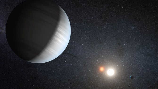
Double Star Systems and their Exoplanets
An artist’s impression of an exoplanet in the Kepler-47 double star system.
Out of the over 800 exoplanets currently known, the majority are found orbiting single stars. However, there are also a significant number of planets that exist in star systems with multiple stars. In fact, recent data reveals that there are 64 exoplanets in double systems.
Exoplanets in double systems can be categorized based on the configuration of their orbits:
- S-class exoplanets orbit around one of the components of the double star system (e.g. OGLE-2013-BLG-0341LB b). There are 57 of these exoplanets.
- P-class exoplanets orbit around both components of the double star system. Examples of these systems include NN Ser, DP Leo, HU Aqr, UZ For, Kepler-16 (AB)b, Kepler-34 (AB)b, and Kepler-35 (AB)b.
When we analyze the data, we can see that:
- A significant proportion of planets exist in systems where the components are spaced between 35 and 100 astronomical units (a.u.), with a particular concentration around the 20 a.u. mark.
- Planets in wide systems (greater than 100 a.u.) have masses ranging from 0.01 to 10 times the mass of Jupiter (MJ), which is similar to the masses of planets around single stars. Conversely, planets in systems with closer separations have masses ranging from 0.1 to 10 MJ.
- Planets in wide systems are always found in isolation.
- The distribution of orbital eccentricities in wide systems differs from that of single planets, often reaching values as high as e = 0.925 and e = 0.935.
Crucial aspects of the formation processes
Disruption of the protoplanetary disk. While in solitary stars the protoplanetary disk can extend up to the Kuiper belt (30-50 a.u.), in binary stars its size is truncated due to the influence of the second component. Consequently, the length of the protoplanetary disk is reduced by 2-5 times compared to the distance between the components.
Deformation of the protoplanetary disk. The remaining disk, after being truncated, continues to be affected by the second component, causing it to stretch, distort, intertwine, and even fracture. This distorted disk also begins to precess.
Reducing the lifespan of a protoplanetary disk. For wide binary systems, similar to single stars, the lifespan of a protoplanetary disk ranges from 1 to 10 million years. However, for systems with a separation of less than 40 a.e., the disk lifespan should be between 0.1 and 1 million years.
Formation scenario of planetesimals
Scenarios of formation without singularity
There exist scenarios where the initial configuration of the planetary system, right after formation, differs from the current one and is achieved through further evolution.
- One such scenario involves the capture of a planet from another star. The interaction cross-section is much larger in a binary star system, increasing the probability of collision and capture of a planet from another star.
- The second scenario suggests that during the evolution of one of the components, after the main sequence in the original planetary system, instabilities occur. This causes the planet to deviate from its original orbit and become shared between both components.
Astronomical data and their analysis
Light curves
Illustrative light curves for a split binary system
Example of light curves for a close binary system
In the case where the binary star is an eclipsing star, it becomes possible to plot the time dependence of the total light. The light variability on this curve will be influenced by:
- The eclipses themselves
- The effects of oblateness
- The effects of reflection, or more accurately, radiation recycling between the stars.
However, analyzing only the eclipses themselves, when the components are spherically symmetric and there are no reflection effects, reduces to solving the following system of equations:
It is not possible to solve this system without making any initial assumptions. Similarly, analyzing more complex scenarios involving ellipsoidal-shaped components and reflection effects, which are crucial in various close double systems, is also not feasible. Hence, all contemporary techniques for analyzing light curves invariably incorporate model assumptions, and the parameters of these assumptions are determined through other types of observations.
Radial velocity curves
When spectroscopically observing a double star, which means it is a spectroscopic double star, it is feasible to create a graph showing the time-dependent changes in the radial velocities of the individual components. Assuming that the orbit is circular, the following equation can be written:
where Vs represents the radial velocity of the component, i is the inclination of the orbit with respect to the line of sight, P is the period, and a is the radius of the component’s orbit. By substituting Kepler’s third law into this equation, we obtain:
where Ms stands for the mass of the component under study, and M2 represents the mass of the second component. Therefore, by observing both components, it is possible to determine the ratio of the masses of the stars that form the double star. If we apply Kepler’s third law again, it can be simplified as follows:
where G is the gravitational constant, and f(M2) represents the mass function of the star and is defined as follows:
In the event that the orbit is not circular but exhibits eccentricity, it can be demonstrated that the mass function must be dominated by a factor of for the orbital period P.
If the second component is not observed, then the function f(M2) acts as a lower limit for its mass.
It is important to note that solely examining the radial velocity curves does not allow for the determination of all the parameters of the double system; there will always be uncertainty in the form of an unknown orbital inclination angle.
Determining the Masses of Components
In most cases, the gravitational interaction between two stars can be adequately described using Newton’s laws and Kepler’s laws, both of which derive from Newton’s laws. However, when studying double pulsars, it becomes necessary to incorporate general relativity. By examining observable effects of relativistic phenomena, it is possible to further verify the accuracy of the theory of relativity.
Kepler’s third law establishes a relationship between the orbital period, the distance between the components, and the total mass of the system:
The orbital period, the major semi-axis of the system, and the masses of the components, as well as the gravitational constant, are all factors that come into play when analyzing a dual system. In cases where the system is visually dual, it is possible to calculate the orbits of both components, as well as determine the period and semi-major axis, and the mass ratio. However, in many instances, the duality of the system can only be determined through spectral data (spectral-double). By analyzing the motion of the spectral lines, it is possible to calculate the radial velocities of one component, and in rare cases, both components. If only the radial velocity of one component is known, it is not possible to obtain complete information about the masses. However, it is still possible to construct a mass function and determine the upper limit of the mass of the second component. This information can then be used to determine whether the second component could potentially be a black hole or a neutron star.